Ver ahora Este tutorial tiene un curso de video relacionado creado por el equipo de Real Python. Míralo junto con el tutorial escrito para profundizar tu comprensión:Lectura y escritura de archivos con Pandas
Pandas es un paquete de Python potente y flexible que le permite trabajar con datos etiquetados y series temporales. También proporciona métodos estadísticos, permite el trazado y más. Una característica crucial de Pandas es su capacidad para escribir y leer Excel, CSV y muchos otros tipos de archivos. Funciones como Pandas read_csv() El método le permite trabajar con archivos de manera efectiva. Puede usarlos para guardar los datos y las etiquetas de los objetos de Pandas en un archivo y cargarlos más tarde como Pandas Series o DataFrame instancias.
En este tutorial, aprenderá:
- Qué son las herramientas Pandas IO La API es
- Cómo leer y escribir datos hacia y desde archivos
- Cómo trabajar con varios formatos de archivo
- Cómo trabajar con grandes datos eficientemente
¡Comencemos a leer y escribir archivos!
Bonificación gratuita: 5 pensamientos sobre el dominio de Python, un curso gratuito para desarrolladores de Python que le muestra la hoja de ruta y la mentalidad que necesitará para llevar sus habilidades de Python al siguiente nivel.
Instalando Pandas
El código de este tutorial se ejecuta con CPython 3.7.4 y Pandas 0.25.1. Sería beneficioso asegurarse de tener las últimas versiones de Python y Pandas en su máquina. Es posible que desee crear un nuevo entorno virtual e instalar las dependencias para este tutorial.
Primero, necesitarás la biblioteca Pandas. Es posible que ya lo tengas instalado. Si no lo hace, puede instalarlo con pip:
$ pip install pandas
Una vez que se completa el proceso de instalación, debe tener Pandas instalado y listo.
Anaconda es una excelente distribución de Python que viene con Python, muchos paquetes útiles como Pandas y un administrador de paquetes y entornos llamado Conda. Para obtener más información sobre Anaconda, consulte Configuración de Python para el aprendizaje automático en Windows.
Si no tiene Pandas en su entorno virtual, puede instalarlo con Conda:
$ conda install pandas
Conda es poderoso ya que administra las dependencias y sus versiones. Para obtener más información sobre cómo trabajar con Conda, puede consultar la documentación oficial.
Preparación de datos
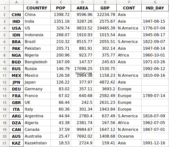
En este tutorial, utilizará los datos relacionados con 20 países. Aquí hay una descripción general de los datos y las fuentes con las que trabajará:
-
País se denota por el nombre del país. Cada país está en la lista de los 10 principales por población, área o producto interno bruto (PIB). Las etiquetas de fila para el conjunto de datos son los códigos de país de tres letras definidos en ISO 3166-1. La etiqueta de la columna para el conjunto de datos es
COUNTRY. -
Población se expresa en millones. Los datos provienen de una lista de países y dependencias por población en Wikipedia. La etiqueta de columna para el conjunto de datos es
POP. -
Área se expresa en miles de kilómetros cuadrados. Los datos provienen de una lista de países y dependencias por área en Wikipedia. La etiqueta de la columna para el conjunto de datos es
AREA. -
Producto interior bruto se expresa en millones de dólares estadounidenses, según datos de las Naciones Unidas para 2017. Puede encontrar estos datos en la lista de países por PIB nominal en Wikipedia. La etiqueta de la columna para el conjunto de datos es
GDP. -
Continente es África, Asia, Oceanía, Europa, América del Norte o América del Sur. También puede encontrar esta información en Wikipedia. La etiqueta de la columna para el conjunto de datos es
CONT. -
Día de la Independencia es una fecha que conmemora la independencia de una nación. Los datos provienen de la lista de días de independencia nacional en Wikipedia. Las fechas se muestran en formato ISO 8601. Los primeros cuatro dígitos representan el año, los siguientes dos números son el mes y los dos últimos son para el día del mes. La etiqueta de columna para el conjunto de datos es
IND_DAY.
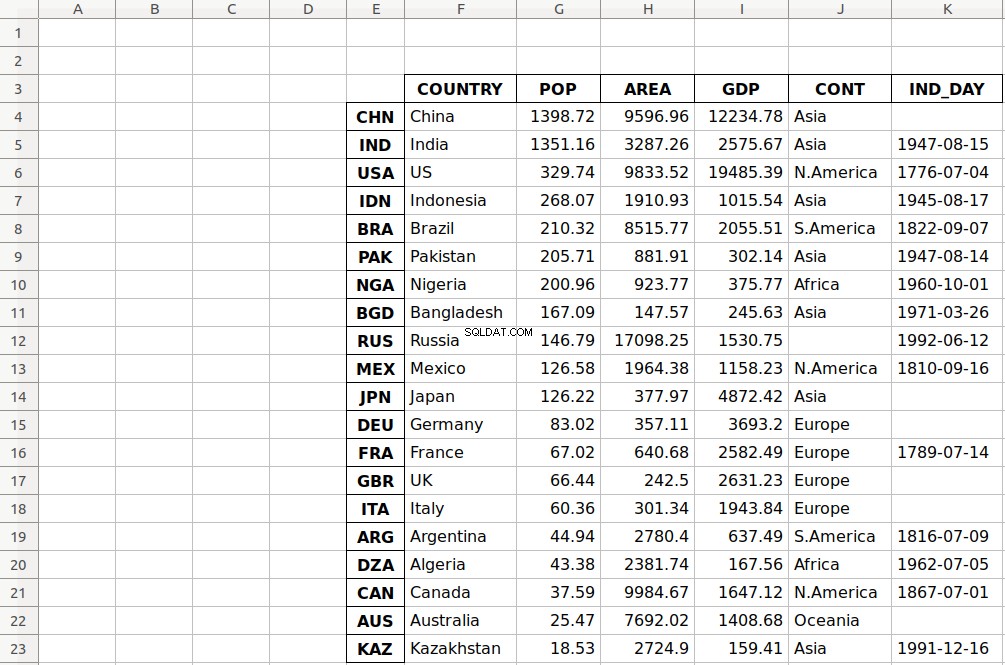
Así es como se ven los datos en una tabla:
| PAÍS | POP | ÁREA | PIB | CONT | IND_DAY | |
|---|---|---|---|---|---|---|
| CHN | China | 1398.72 | 9596.96 | 12234.78 | Asia | |
| IND | India | 1351.16 | 3287.26 | 2575.67 | Asia | 1947-08-15 |
| EE.UU. | EE.UU. | 329,74 | 9833.52 | 19485.39 | Norteamérica | 1776-07-04 |
| IDN | Indonesia | 268.07 | 1910.93 | 1015.54 | Asia | 1945-08-17 |
| SUJETADOR | Brasil | 210.32 | 8515.77 | 2055.51 | S. América | 1822-09-07 |
| PAK | Pakistán | 205.71 | 881.91 | 302.14 | Asia | 1947-08-14 |
| NGA | Nigeria | 200,96 | 923,77 | 375,77 | África | 1960-10-01 |
| BGD | Bangladesh | 167.09 | 147,57 | 245,63 | Asia | 1971-03-26 |
| RUS | Rusia | 146,79 | 17098.25 | 1530,75 | 12-06-1992 | |
| MEX | México | 126,58 | 1964.38 | 1158.23 | Norteamérica | 1810-09-16 |
| JPN | Japón | 126,22 | 377,97 | 4872.42 | Asia | |
| DEU | Alemania | 83.02 | 357.11 | 3693.20 | Europa | |
| FRA | Francia | 67.02 | 640,68 | 2582.49 | Europa | 1789-07-14 |
| GBR | Reino Unido | 66,44 | 242,50 | 2631.23 | Europa | |
| ITA | Italia | 60,36 | 301.34 | 1943.84 | Europa | |
| ARG | Argentina | 44,94 | 2780.40 | 637,49 | S. América | 1816-07-09 |
| DZA | Argelia | 43,38 | 2381.74 | 167,56 | África | 1962-07-05 |
| PUEDE | Canadá | 37,59 | 9984.67 | 1647.12 | Norteamérica | 1867-07-01 |
| AUS | Australia | 25,47 | 7692.02 | 1408.68 | Oceanía | |
| KAZ | Kazajistán | 18.53 | 2724.90 | 159,41 | Asia | 1991-12-16 |
Puede notar que faltan algunos de los datos. Por ejemplo, el continente de Rusia no se especifica porque se extiende por Europa y Asia. También faltan varios días de independencia porque la fuente de datos los omite.
Puede organizar estos datos en Python usando un diccionario anidado:
data = {
    'CHN': {'COUNTRY': 'China', 'POP': 1_398.72, 'AREA': 9_596.96,
            'GDP': 12_234.78, 'CONT': 'Asia'},
    'IND': {'COUNTRY': 'India', 'POP': 1_351.16, 'AREA': 3_287.26,
            'GDP': 2_575.67, 'CONT': 'Asia', 'IND_DAY': '1947-08-15'},
    'USA': {'COUNTRY': 'US', 'POP': 329.74, 'AREA': 9_833.52,
            'GDP': 19_485.39, 'CONT': 'N.America',
            'IND_DAY': '1776-07-04'},
    'IDN': {'COUNTRY': 'Indonesia', 'POP': 268.07, 'AREA': 1_910.93,
            'GDP': 1_015.54, 'CONT': 'Asia', 'IND_DAY': '1945-08-17'},
    'BRA': {'COUNTRY': 'Brazil', 'POP': 210.32, 'AREA': 8_515.77,
            'GDP': 2_055.51, 'CONT': 'S.America', 'IND_DAY': '1822-09-07'},
    'PAK': {'COUNTRY': 'Pakistan', 'POP': 205.71, 'AREA': 881.91,
            'GDP': 302.14, 'CONT': 'Asia', 'IND_DAY': '1947-08-14'},
    'NGA': {'COUNTRY': 'Nigeria', 'POP': 200.96, 'AREA': 923.77,
            'GDP': 375.77, 'CONT': 'Africa', 'IND_DAY': '1960-10-01'},
    'BGD': {'COUNTRY': 'Bangladesh', 'POP': 167.09, 'AREA': 147.57,
            'GDP': 245.63, 'CONT': 'Asia', 'IND_DAY': '1971-03-26'},
    'RUS': {'COUNTRY': 'Russia', 'POP': 146.79, 'AREA': 17_098.25,
            'GDP': 1_530.75, 'IND_DAY': '1992-06-12'},
    'MEX': {'COUNTRY': 'Mexico', 'POP': 126.58, 'AREA': 1_964.38,
            'GDP': 1_158.23, 'CONT': 'N.America', 'IND_DAY': '1810-09-16'},
    'JPN': {'COUNTRY': 'Japan', 'POP': 126.22, 'AREA': 377.97,
            'GDP': 4_872.42, 'CONT': 'Asia'},
    'DEU': {'COUNTRY': 'Germany', 'POP': 83.02, 'AREA': 357.11,
            'GDP': 3_693.20, 'CONT': 'Europe'},
    'FRA': {'COUNTRY': 'France', 'POP': 67.02, 'AREA': 640.68,
            'GDP': 2_582.49, 'CONT': 'Europe', 'IND_DAY': '1789-07-14'},
    'GBR': {'COUNTRY': 'UK', 'POP': 66.44, 'AREA': 242.50,
            'GDP': 2_631.23, 'CONT': 'Europe'},
    'ITA': {'COUNTRY': 'Italy', 'POP': 60.36, 'AREA': 301.34,
            'GDP': 1_943.84, 'CONT': 'Europe'},
    'ARG': {'COUNTRY': 'Argentina', 'POP': 44.94, 'AREA': 2_780.40,
            'GDP': 637.49, 'CONT': 'S.America', 'IND_DAY': '1816-07-09'},
    'DZA': {'COUNTRY': 'Algeria', 'POP': 43.38, 'AREA': 2_381.74,
            'GDP': 167.56, 'CONT': 'Africa', 'IND_DAY': '1962-07-05'},
    'CAN': {'COUNTRY': 'Canada', 'POP': 37.59, 'AREA': 9_984.67,
            'GDP': 1_647.12, 'CONT': 'N.America', 'IND_DAY': '1867-07-01'},
    'AUS': {'COUNTRY': 'Australia', 'POP': 25.47, 'AREA': 7_692.02,
            'GDP': 1_408.68, 'CONT': 'Oceania'},
    'KAZ': {'COUNTRY': 'Kazakhstan', 'POP': 18.53, 'AREA': 2_724.90,
            'GDP': 159.41, 'CONT': 'Asia', 'IND_DAY': '1991-12-16'}
}

columns = ('COUNTRY', 'POP', 'AREA', 'GDP', 'CONT', 'IND_DAY')
Cada fila de la tabla está escrita como un diccionario interno cuyas claves son los nombres de las columnas y los valores son los datos correspondientes. Estos diccionarios luego se recopilan como los valores en los data externos diccionario. Las claves correspondientes para data son los códigos de país de tres letras.
Puedes usar estos data para crear una instancia de Pandas DataFrame . Primero, necesitas importar Pandas:
>>> import pandas as pd
Ahora que ha importado Pandas, puede usar el DataFrame constructor y data para crear un DataFrame objeto.
data está organizado de tal manera que los códigos de país corresponden a columnas. Puede invertir las filas y columnas de un DataFrame con la propiedad .T :
>>> df = pd.DataFrame(data=data).T
>>> df
        COUNTRY      POP     AREA      GDP       CONT     IND_DAY
CHN       China  1398.72  9596.96  12234.8       Asia         NaN
IND       India  1351.16  3287.26  2575.67       Asia  1947-08-15
USA          US   329.74  9833.52  19485.4  N.America  1776-07-04
IDN   Indonesia   268.07  1910.93  1015.54       Asia  1945-08-17
BRA      Brazil   210.32  8515.77  2055.51  S.America  1822-09-07
PAK    Pakistan   205.71   881.91   302.14       Asia  1947-08-14
NGA     Nigeria   200.96   923.77   375.77     Africa  1960-10-01
BGD  Bangladesh   167.09   147.57   245.63       Asia  1971-03-26
RUS      Russia   146.79  17098.2  1530.75        NaN  1992-06-12
MEX      Mexico   126.58  1964.38  1158.23  N.America  1810-09-16
JPN       Japan   126.22   377.97  4872.42       Asia         NaN
DEU     Germany    83.02   357.11   3693.2     Europe         NaN
FRA      France    67.02   640.68  2582.49     Europe  1789-07-14
GBR          UK    66.44    242.5  2631.23     Europe         NaN
ITA       Italy    60.36   301.34  1943.84     Europe         NaN
ARG   Argentina    44.94   2780.4   637.49  S.America  1816-07-09
DZA     Algeria    43.38  2381.74   167.56     Africa  1962-07-05
CAN      Canada    37.59  9984.67  1647.12  N.America  1867-07-01
AUS   Australia    25.47  7692.02  1408.68    Oceania         NaN
KAZ  Kazakhstan    18.53   2724.9   159.41       Asia  1991-12-16
Ahora tienes tu DataFrame objeto poblado con los datos de cada país.
.transpose() en lugar de .T para invertir las filas y columnas de su conjunto de datos. Si usa .transpose() , luego puede configurar el parámetro opcional copy para especificar si desea copiar los datos subyacentes. El comportamiento predeterminado es False .
Las versiones de Python anteriores a la 3.6 no garantizaban el orden de las claves en los diccionarios. Para garantizar que se mantenga el orden de las columnas para versiones anteriores de Python y Pandas, puede especificar index=columns :
>>> df = pd.DataFrame(data=data, index=columns).T
Ahora que ha preparado sus datos, ¡está listo para comenzar a trabajar con archivos!
Uso de Pandas read_csv() y .to_csv() Funciones
Un archivo de valores separados por comas (CSV) es un archivo de texto sin formato con un .csv extensión que contiene datos tabulares. Este es uno de los formatos de archivo más populares para almacenar grandes cantidades de datos. Cada fila del archivo CSV representa una única fila de la tabla. Los valores en la misma fila están separados por comas de manera predeterminada, pero puede cambiar el separador a punto y coma, tabulación, espacio o algún otro carácter.
Escribir un archivo CSV
Puedes guardar tu Pandas DataFrame como archivo CSV con .to_csv() :
>>> df.to_csv('data.csv')
¡Eso es todo! Ha creado el archivo data.csv en su directorio de trabajo actual. Puede expandir el bloque de código a continuación para ver cómo debería verse su archivo CSV:
,COUNTRY,POP,AREA,GDP,CONT,IND_DAY
CHN,China,1398.72,9596.96,12234.78,Asia,
IND,India,1351.16,3287.26,2575.67,Asia,1947-08-15
USA,US,329.74,9833.52,19485.39,N.America,1776-07-04
IDN,Indonesia,268.07,1910.93,1015.54,Asia,1945-08-17
BRA,Brazil,210.32,8515.77,2055.51,S.America,1822-09-07
PAK,Pakistan,205.71,881.91,302.14,Asia,1947-08-14
NGA,Nigeria,200.96,923.77,375.77,Africa,1960-10-01
BGD,Bangladesh,167.09,147.57,245.63,Asia,1971-03-26
RUS,Russia,146.79,17098.25,1530.75,,1992-06-12
MEX,Mexico,126.58,1964.38,1158.23,N.America,1810-09-16
JPN,Japan,126.22,377.97,4872.42,Asia,
DEU,Germany,83.02,357.11,3693.2,Europe,
FRA,France,67.02,640.68,2582.49,Europe,1789-07-14
GBR,UK,66.44,242.5,2631.23,Europe,
ITA,Italy,60.36,301.34,1943.84,Europe,
ARG,Argentina,44.94,2780.4,637.49,S.America,1816-07-09
DZA,Algeria,43.38,2381.74,167.56,Africa,1962-07-05
CAN,Canada,37.59,9984.67,1647.12,N.America,1867-07-01
AUS,Australia,25.47,7692.02,1408.68,Oceania,
KAZ,Kazakhstan,18.53,2724.9,159.41,Asia,1991-12-16
Este archivo de texto contiene los datos separados por comas . La primera columna contiene las etiquetas de las filas. En algunos casos, los encontrará irrelevantes. Si no desea mantenerlos, puede pasar el argumento index=False a .to_csv() .
Leer un archivo CSV
Una vez que sus datos se guardan en un archivo CSV, es probable que desee cargarlos y usarlos de vez en cuando. Puedes hacer eso con Pandas read_csv() función:
>>> df = pd.read_csv('data.csv', index_col=0)
>>> df
        COUNTRY      POP      AREA       GDP       CONT     IND_DAY
CHN       China  1398.72   9596.96  12234.78       Asia         NaN
IND       India  1351.16   3287.26   2575.67       Asia  1947-08-15
USA          US   329.74   9833.52  19485.39  N.America  1776-07-04
IDN   Indonesia   268.07   1910.93   1015.54       Asia  1945-08-17
BRA      Brazil   210.32   8515.77   2055.51  S.America  1822-09-07
PAK    Pakistan   205.71    881.91    302.14       Asia  1947-08-14
NGA     Nigeria   200.96    923.77    375.77     Africa  1960-10-01
BGD  Bangladesh   167.09    147.57    245.63       Asia  1971-03-26
RUS      Russia   146.79  17098.25   1530.75        NaN  1992-06-12
MEX      Mexico   126.58   1964.38   1158.23  N.America  1810-09-16
JPN       Japan   126.22    377.97   4872.42       Asia         NaN
DEU     Germany    83.02    357.11   3693.20     Europe         NaN
FRA      France    67.02    640.68   2582.49     Europe  1789-07-14
GBR          UK    66.44    242.50   2631.23     Europe         NaN
ITA       Italy    60.36    301.34   1943.84     Europe         NaN
ARG   Argentina    44.94   2780.40    637.49  S.America  1816-07-09
DZA     Algeria    43.38   2381.74    167.56     Africa  1962-07-05
CAN      Canada    37.59   9984.67   1647.12  N.America  1867-07-01
AUS   Australia    25.47   7692.02   1408.68    Oceania         NaN
KAZ  Kazakhstan    18.53   2724.90    159.41       Asia  1991-12-16
En este caso, los Pandas read_csv() la función devuelve un nuevo DataFrame con los datos y etiquetas del archivo data.csv , que especificó con el primer argumento. Esta cadena puede ser cualquier ruta válida, incluidas las URL.
El parámetro index_col especifica la columna del archivo CSV que contiene las etiquetas de fila. Asigne un índice de columna de base cero a este parámetro. Debe determinar el valor de index_col cuando el archivo CSV contiene las etiquetas de las filas para evitar cargarlas como datos.
Aprenderá más sobre el uso de Pandas con archivos CSV más adelante en este tutorial. También puede consultar Lectura y escritura de archivos CSV en Python para ver cómo manejar archivos CSV con la biblioteca integrada de Python csv también.
Uso de Pandas para escribir y leer archivos de Excel
Microsoft Excel es probablemente el software de hoja de cálculo más utilizado. Mientras que las versiones anteriores usaban .xls binario archivos, Excel 2007 introdujo el nuevo .xlsx basado en XML expediente. Puede leer y escribir archivos de Excel en Pandas, de forma similar a los archivos CSV. Sin embargo, primero deberá instalar los siguientes paquetes de Python:
- xlwt para escribir en
.xlsarchivos - openpyxl o XlsxWriter para escribir en
.xlsxarchivos - xlrd para leer archivos de Excel
Puede instalarlos usando pip con un solo comando:
$ pip install xlwt openpyxl xlsxwriter xlrd
También puedes usar Conda:
$ conda install xlwt openpyxl xlsxwriter xlrd
Tenga en cuenta que no tiene que instalar todos estos paquetes. Por ejemplo, no necesita tanto openpyxl como XlsxWriter. Si vas a trabajar solo con .xls archivos, entonces no necesita ninguno de ellos! Sin embargo, si tiene la intención de trabajar solo con .xlsx archivos, necesitará al menos uno de ellos, pero no xlwt . Tómese su tiempo para decidir qué paquetes son adecuados para su proyecto.
Escribir un archivo de Excel
Una vez que haya instalado esos paquetes, puede guardar su DataFrame en un archivo de Excel con .to_excel() :
>>> df.to_excel('data.xlsx')
El argumento 'data.xlsx' representa el archivo de destino y, opcionalmente, su ruta. La declaración anterior debería crear el archivo data.xlsx en su directorio de trabajo actual. Ese archivo debería verse así:
La primera columna del archivo contiene las etiquetas de las filas, mientras que las otras columnas almacenan datos.
Leer un archivo de Excel
Puede cargar datos de archivos de Excel con read_excel() :
>>> df = pd.read_excel('data.xlsx', index_col=0)
>>> df
        COUNTRY      POP      AREA       GDP       CONT     IND_DAY
CHN       China  1398.72   9596.96  12234.78       Asia         NaN
IND       India  1351.16   3287.26   2575.67       Asia  1947-08-15
USA          US   329.74   9833.52  19485.39  N.America  1776-07-04
IDN   Indonesia   268.07   1910.93   1015.54       Asia  1945-08-17
BRA      Brazil   210.32   8515.77   2055.51  S.America  1822-09-07
PAK    Pakistan   205.71    881.91    302.14       Asia  1947-08-14
NGA     Nigeria   200.96    923.77    375.77     Africa  1960-10-01
BGD  Bangladesh   167.09    147.57    245.63       Asia  1971-03-26
RUS      Russia   146.79  17098.25   1530.75        NaN  1992-06-12
MEX      Mexico   126.58   1964.38   1158.23  N.America  1810-09-16
JPN       Japan   126.22    377.97   4872.42       Asia         NaN
DEU     Germany    83.02    357.11   3693.20     Europe         NaN
FRA      France    67.02    640.68   2582.49     Europe  1789-07-14
GBR          UK    66.44    242.50   2631.23     Europe         NaN
ITA       Italy    60.36    301.34   1943.84     Europe         NaN
ARG   Argentina    44.94   2780.40    637.49  S.America  1816-07-09
DZA     Algeria    43.38   2381.74    167.56     Africa  1962-07-05
CAN      Canada    37.59   9984.67   1647.12  N.America  1867-07-01
AUS   Australia    25.47   7692.02   1408.68    Oceania         NaN
KAZ  Kazakhstan    18.53   2724.90    159.41       Asia  1991-12-16
read_excel() devuelve un nuevo DataFrame que contiene los valores de data.xlsx . También puede usar read_excel() con hojas de cálculo OpenDocument, o .ods archivos.
Aprenderá más sobre cómo trabajar con archivos de Excel más adelante en este tutorial. También puede consultar Uso de pandas para leer archivos grandes de Excel en Python.
Comprender la API de Pandas IO
Herramientas de E/S de Pandas es la API que te permite guardar el contenido de Series y DataFrame objetos al portapapeles, objetos o archivos de varios tipos. También permite cargar datos desde el portapapeles, objetos o archivos.
Escribir archivos
Series y DataFrame los objetos tienen métodos que permiten escribir datos y etiquetas en el portapapeles o en los archivos. Se nombran con el patrón .to_<file-type>() , donde <file-type> es el tipo del archivo de destino.
Has aprendido sobre .to_csv() y .to_excel() , pero hay otros, incluyendo:
.to_json().to_html().to_sql().to_pickle()
Todavía hay más tipos de archivos en los que puede escribir, por lo que esta lista no es exhaustiva.
Series y DataFrame objetos.
Estos métodos tienen parámetros que especifican la ruta del archivo de destino donde guardó los datos y las etiquetas. Esto es obligatorio en algunos casos y opcional en otros. Si esta opción está disponible y elige omitirla, los métodos devolverán los objetos (como cadenas o iterables) con el contenido de DataFrame instancias.
El parámetro opcional compression decide cómo comprimir el archivo con los datos y las etiquetas. Aprenderás más sobre esto más adelante. Hay algunos otros parámetros, pero en su mayoría son específicos de uno o varios métodos. No entrará en ellos en detalle aquí.
Leer archivos
Las funciones de Pandas para leer el contenido de los archivos se nombran usando el patrón .read_<file-type>() , donde <file-type> indica el tipo de archivo a leer. Ya has visto los Pandas read_csv() y read_excel() funciones Aquí hay algunos otros:
read_json()read_html()read_sql()read_pickle()
Estas funciones tienen un parámetro que especifica la ruta del archivo de destino. Puede ser cualquier cadena válida que represente la ruta, ya sea en una máquina local o en una URL. Otros objetos también son aceptables según el tipo de archivo.
El parámetro opcional compression determina el tipo de descompresión a usar para los archivos comprimidos. Lo aprenderá más adelante en este tutorial. Hay otros parámetros, pero son específicos de una o varias funciones. No entrará en ellos en detalle aquí.
Trabajar con diferentes tipos de archivos
La biblioteca de Pandas ofrece una amplia gama de posibilidades para guardar sus datos en archivos y cargar datos desde archivos. En esta sección, obtendrá más información sobre cómo trabajar con archivos CSV y Excel. También verá cómo usar otros tipos de archivos, como JSON, páginas web, bases de datos y archivos pickle de Python.
Archivos CSV
Ya aprendió a leer y escribir archivos CSV. Ahora profundicemos un poco más en los detalles. Cuando usas .to_csv() para guardar su DataFrame , puede proporcionar un argumento para el parámetro path_or_buf para especificar la ruta, el nombre y la extensión del archivo de destino.
path_or_buf es el primer argumento .to_csv() obtendrá. Puede ser cualquier cadena que represente una ruta de archivo válida que incluya el nombre del archivo y su extensión. Lo has visto en un ejemplo anterior. Sin embargo, si omite path_or_buf , luego .to_csv() no creará ningún archivo. En su lugar, devolverá la cadena correspondiente:
>>> df = pd.DataFrame(data=data).T
>>> s = df.to_csv()
>>> print(s)
,COUNTRY,POP,AREA,GDP,CONT,IND_DAY
CHN,China,1398.72,9596.96,12234.78,Asia,
IND,India,1351.16,3287.26,2575.67,Asia,1947-08-15
USA,US,329.74,9833.52,19485.39,N.America,1776-07-04
IDN,Indonesia,268.07,1910.93,1015.54,Asia,1945-08-17
BRA,Brazil,210.32,8515.77,2055.51,S.America,1822-09-07
PAK,Pakistan,205.71,881.91,302.14,Asia,1947-08-14
NGA,Nigeria,200.96,923.77,375.77,Africa,1960-10-01
BGD,Bangladesh,167.09,147.57,245.63,Asia,1971-03-26
RUS,Russia,146.79,17098.25,1530.75,,1992-06-12
MEX,Mexico,126.58,1964.38,1158.23,N.America,1810-09-16
JPN,Japan,126.22,377.97,4872.42,Asia,
DEU,Germany,83.02,357.11,3693.2,Europe,
FRA,France,67.02,640.68,2582.49,Europe,1789-07-14
GBR,UK,66.44,242.5,2631.23,Europe,
ITA,Italy,60.36,301.34,1943.84,Europe,
ARG,Argentina,44.94,2780.4,637.49,S.America,1816-07-09
DZA,Algeria,43.38,2381.74,167.56,Africa,1962-07-05
CAN,Canada,37.59,9984.67,1647.12,N.America,1867-07-01
AUS,Australia,25.47,7692.02,1408.68,Oceania,
KAZ,Kazakhstan,18.53,2724.9,159.41,Asia,1991-12-16
Ahora tienes la cadena s en lugar de un archivo CSV. También tiene algunos valores perdidos en su DataFrame objeto. Por ejemplo, el continente de Rusia y los días de la independencia de varios países (China, Japón, etc.) no están disponibles. En ciencia de datos y aprendizaje automático, debe manejar los valores faltantes con cuidado. ¡Pandas sobresale aquí! De forma predeterminada, Pandas usa el valor de NaN para reemplazar los valores que faltan.
nan , que significa "no es un número", es un valor particular de coma flotante en Python.
Puedes obtener un nan valor con cualquiera de las siguientes funciones:
float('nan')math.nannumpy.nan
El continente que corresponde a Rusia en df es nan :
>>> df.loc['RUS', 'CONT']
nan
Este ejemplo usa .loc[] para obtener datos con los nombres de fila y columna especificados.
Cuando guardas tu DataFrame a un archivo CSV, cadenas vacías ('' ) representará los datos faltantes. Puede ver esto en su archivo data.csv y en la cadena s . Si desea cambiar este comportamiento, utilice el parámetro opcional na_rep :
>>> df.to_csv('new-data.csv', na_rep='(missing)')
Este código produce el archivo new-data.csv donde los valores que faltan ya no son cadenas vacías. Puede expandir el bloque de código a continuación para ver cómo debería verse este archivo:
,COUNTRY,POP,AREA,GDP,CONT,IND_DAY
CHN,China,1398.72,9596.96,12234.78,Asia,(missing)
IND,India,1351.16,3287.26,2575.67,Asia,1947-08-15
USA,US,329.74,9833.52,19485.39,N.America,1776-07-04
IDN,Indonesia,268.07,1910.93,1015.54,Asia,1945-08-17
BRA,Brazil,210.32,8515.77,2055.51,S.America,1822-09-07
PAK,Pakistan,205.71,881.91,302.14,Asia,1947-08-14
NGA,Nigeria,200.96,923.77,375.77,Africa,1960-10-01
BGD,Bangladesh,167.09,147.57,245.63,Asia,1971-03-26
RUS,Russia,146.79,17098.25,1530.75,(missing),1992-06-12
MEX,Mexico,126.58,1964.38,1158.23,N.America,1810-09-16
JPN,Japan,126.22,377.97,4872.42,Asia,(missing)
DEU,Germany,83.02,357.11,3693.2,Europe,(missing)
FRA,France,67.02,640.68,2582.49,Europe,1789-07-14
GBR,UK,66.44,242.5,2631.23,Europe,(missing)
ITA,Italy,60.36,301.34,1943.84,Europe,(missing)
ARG,Argentina,44.94,2780.4,637.49,S.America,1816-07-09
DZA,Algeria,43.38,2381.74,167.56,Africa,1962-07-05
CAN,Canada,37.59,9984.67,1647.12,N.America,1867-07-01
AUS,Australia,25.47,7692.02,1408.68,Oceania,(missing)
KAZ,Kazakhstan,18.53,2724.9,159.41,Asia,1991-12-16
Now, the string '(missing)' in the file corresponds to the nan values from df .
When Pandas reads files, it considers the empty string ('' ) and a few others as missing values by default:
'nan''-nan''NA''N/A''NaN''null'
If you don’t want this behavior, then you can pass keep_default_na=False to the Pandas read_csv() función. To specify other labels for missing values, use the parameter na_values :
>>> pd.read_csv('new-data.csv', index_col=0, na_values='(missing)')
        COUNTRY      POP      AREA       GDP       CONT     IND_DAY
CHN       China  1398.72   9596.96  12234.78       Asia         NaN
IND       India  1351.16   3287.26   2575.67       Asia  1947-08-15
USA          US   329.74   9833.52  19485.39  N.America  1776-07-04
IDN   Indonesia   268.07   1910.93   1015.54       Asia  1945-08-17
BRA      Brazil   210.32   8515.77   2055.51  S.America  1822-09-07
PAK    Pakistan   205.71    881.91    302.14       Asia  1947-08-14
NGA     Nigeria   200.96    923.77    375.77     Africa  1960-10-01
BGD  Bangladesh   167.09    147.57    245.63       Asia  1971-03-26
RUS      Russia   146.79  17098.25   1530.75        NaN  1992-06-12
MEX      Mexico   126.58   1964.38   1158.23  N.America  1810-09-16
JPN       Japan   126.22    377.97   4872.42       Asia         NaN
DEU     Germany    83.02    357.11   3693.20     Europe         NaN
FRA      France    67.02    640.68   2582.49     Europe  1789-07-14
GBR          UK    66.44    242.50   2631.23     Europe         NaN
ITA       Italy    60.36    301.34   1943.84     Europe         NaN
ARG   Argentina    44.94   2780.40    637.49  S.America  1816-07-09
DZA     Algeria    43.38   2381.74    167.56     Africa  1962-07-05
CAN      Canada    37.59   9984.67   1647.12  N.America  1867-07-01
AUS   Australia    25.47   7692.02   1408.68    Oceania         NaN
KAZ  Kazakhstan    18.53   2724.90    159.41       Asia  1991-12-16
Here, you’ve marked the string '(missing)' as a new missing data label, and Pandas replaced it with nan when it read the file.
When you load data from a file, Pandas assigns the data types to the values of each column by default. You can check these types with .dtypes :
>>> df = pd.read_csv('data.csv', index_col=0)
>>> df.dtypes
COUNTRY     object
POP        float64
AREA       float64
GDP        float64
CONT        object
IND_DAY     object
dtype: object
The columns with strings and dates ('COUNTRY' , 'CONT' , and 'IND_DAY' ) have the data type object . Meanwhile, the numeric columns contain 64-bit floating-point numbers (float64 ).
You can use the parameter dtype to specify the desired data types and parse_dates to force use of datetimes:
>>> dtypes = {'POP': 'float32', 'AREA': 'float32', 'GDP': 'float32'}
>>> df = pd.read_csv('data.csv', index_col=0, dtype=dtypes,
...                  parse_dates=['IND_DAY'])
>>> df.dtypes
COUNTRY            object
POP               float32
AREA              float32
GDP               float32
CONT               object
IND_DAY    datetime64[ns]
dtype: object
>>> df['IND_DAY']
CHN          NaT
IND   1947-08-15
USA   1776-07-04
IDN   1945-08-17
BRA   1822-09-07
PAK   1947-08-14
NGA   1960-10-01
BGD   1971-03-26
RUS   1992-06-12
MEX   1810-09-16
JPN          NaT
DEU          NaT
FRA   1789-07-14
GBR          NaT
ITA          NaT
ARG   1816-07-09
DZA   1962-07-05
CAN   1867-07-01
AUS          NaT
KAZ   1991-12-16
Name: IND_DAY, dtype: datetime64[ns]
Now, you have 32-bit floating-point numbers (float32 ) as specified with dtype . These differ slightly from the original 64-bit numbers because of smaller precision . The values in the last column are considered as dates and have the data type datetime64 . That’s why the NaN values in this column are replaced with NaT .
Now that you have real dates, you can save them in the format you like:
>>>>>> df = pd.read_csv('data.csv', index_col=0, parse_dates=['IND_DAY'])
>>> df.to_csv('formatted-data.csv', date_format='%B %d, %Y')
Here, you’ve specified the parameter date_format to be '%B %d, %Y' . You can expand the code block below to see the resulting file:
,COUNTRY,POP,AREA,GDP,CONT,IND_DAY
CHN,China,1398.72,9596.96,12234.78,Asia,
IND,India,1351.16,3287.26,2575.67,Asia,"August 15, 1947"
USA,US,329.74,9833.52,19485.39,N.America,"July 04, 1776"
IDN,Indonesia,268.07,1910.93,1015.54,Asia,"August 17, 1945"
BRA,Brazil,210.32,8515.77,2055.51,S.America,"September 07, 1822"
PAK,Pakistan,205.71,881.91,302.14,Asia,"August 14, 1947"
NGA,Nigeria,200.96,923.77,375.77,Africa,"October 01, 1960"
BGD,Bangladesh,167.09,147.57,245.63,Asia,"March 26, 1971"
RUS,Russia,146.79,17098.25,1530.75,,"June 12, 1992"
MEX,Mexico,126.58,1964.38,1158.23,N.America,"September 16, 1810"
JPN,Japan,126.22,377.97,4872.42,Asia,
DEU,Germany,83.02,357.11,3693.2,Europe,
FRA,France,67.02,640.68,2582.49,Europe,"July 14, 1789"
GBR,UK,66.44,242.5,2631.23,Europe,
ITA,Italy,60.36,301.34,1943.84,Europe,
ARG,Argentina,44.94,2780.4,637.49,S.America,"July 09, 1816"
DZA,Algeria,43.38,2381.74,167.56,Africa,"July 05, 1962"
CAN,Canada,37.59,9984.67,1647.12,N.America,"July 01, 1867"
AUS,Australia,25.47,7692.02,1408.68,Oceania,
KAZ,Kazakhstan,18.53,2724.9,159.41,Asia,"December 16, 1991"
The format of the dates is different now. The format '%B %d, %Y' means the date will first display the full name of the month, then the day followed by a comma, and finally the full year.
There are several other optional parameters that you can use with .to_csv() :
sepdenotes a values separator.decimalindicates a decimal separator.encodingsets the file encoding.headerspecifies whether you want to write column labels in the file.
Here’s how you would pass arguments for sep and header :
>>> s = df.to_csv(sep=';', header=False)
>>> print(s)
CHN;China;1398.72;9596.96;12234.78;Asia;
IND;India;1351.16;3287.26;2575.67;Asia;1947-08-15
USA;US;329.74;9833.52;19485.39;N.America;1776-07-04
IDN;Indonesia;268.07;1910.93;1015.54;Asia;1945-08-17
BRA;Brazil;210.32;8515.77;2055.51;S.America;1822-09-07
PAK;Pakistan;205.71;881.91;302.14;Asia;1947-08-14
NGA;Nigeria;200.96;923.77;375.77;Africa;1960-10-01
BGD;Bangladesh;167.09;147.57;245.63;Asia;1971-03-26
RUS;Russia;146.79;17098.25;1530.75;;1992-06-12
MEX;Mexico;126.58;1964.38;1158.23;N.America;1810-09-16
JPN;Japan;126.22;377.97;4872.42;Asia;
DEU;Germany;83.02;357.11;3693.2;Europe;
FRA;France;67.02;640.68;2582.49;Europe;1789-07-14
GBR;UK;66.44;242.5;2631.23;Europe;
ITA;Italy;60.36;301.34;1943.84;Europe;
ARG;Argentina;44.94;2780.4;637.49;S.America;1816-07-09
DZA;Algeria;43.38;2381.74;167.56;Africa;1962-07-05
CAN;Canada;37.59;9984.67;1647.12;N.America;1867-07-01
AUS;Australia;25.47;7692.02;1408.68;Oceania;
KAZ;Kazakhstan;18.53;2724.9;159.41;Asia;1991-12-16
The data is separated with a semicolon (';' ) because you’ve specified sep=';' . Also, since you passed header=False , you see your data without the header row of column names.
The Pandas read_csv() function has many additional options for managing missing data, working with dates and times, quoting, encoding, handling errors, and more. For instance, if you have a file with one data column and want to get a Series object instead of a DataFrame , then you can pass squeeze=True to read_csv() . You’ll learn later on about data compression and decompression, as well as how to skip rows and columns.
JSON Files
JSON stands for JavaScript object notation. JSON files are plaintext files used for data interchange, and humans can read them easily. They follow the ISO/IEC 21778:2017 and ECMA-404 standards and use the .json extensión. Python and Pandas work well with JSON files, as Python’s json library offers built-in support for them.
You can save the data from your DataFrame to a JSON file with .to_json() . Start by creating a DataFrame object again. Use the dictionary data that holds the data about countries and then apply .to_json() :
>>> df = pd.DataFrame(data=data).T
>>> df.to_json('data-columns.json')
This code produces the file data-columns.json . You can expand the code block below to see how this file should look:
{"COUNTRY":{"CHN":"China","IND":"India","USA":"US","IDN":"Indonesia","BRA":"Brazil","PAK":"Pakistan","NGA":"Nigeria","BGD":"Bangladesh","RUS":"Russia","MEX":"Mexico","JPN":"Japan","DEU":"Germany","FRA":"France","GBR":"UK","ITA":"Italy","ARG":"Argentina","DZA":"Algeria","CAN":"Canada","AUS":"Australia","KAZ":"Kazakhstan"},"POP":{"CHN":1398.72,"IND":1351.16,"USA":329.74,"IDN":268.07,"BRA":210.32,"PAK":205.71,"NGA":200.96,"BGD":167.09,"RUS":146.79,"MEX":126.58,"JPN":126.22,"DEU":83.02,"FRA":67.02,"GBR":66.44,"ITA":60.36,"ARG":44.94,"DZA":43.38,"CAN":37.59,"AUS":25.47,"KAZ":18.53},"AREA":{"CHN":9596.96,"IND":3287.26,"USA":9833.52,"IDN":1910.93,"BRA":8515.77,"PAK":881.91,"NGA":923.77,"BGD":147.57,"RUS":17098.25,"MEX":1964.38,"JPN":377.97,"DEU":357.11,"FRA":640.68,"GBR":242.5,"ITA":301.34,"ARG":2780.4,"DZA":2381.74,"CAN":9984.67,"AUS":7692.02,"KAZ":2724.9},"GDP":{"CHN":12234.78,"IND":2575.67,"USA":19485.39,"IDN":1015.54,"BRA":2055.51,"PAK":302.14,"NGA":375.77,"BGD":245.63,"RUS":1530.75,"MEX":1158.23,"JPN":4872.42,"DEU":3693.2,"FRA":2582.49,"GBR":2631.23,"ITA":1943.84,"ARG":637.49,"DZA":167.56,"CAN":1647.12,"AUS":1408.68,"KAZ":159.41},"CONT":{"CHN":"Asia","IND":"Asia","USA":"N.America","IDN":"Asia","BRA":"S.America","PAK":"Asia","NGA":"Africa","BGD":"Asia","RUS":null,"MEX":"N.America","JPN":"Asia","DEU":"Europe","FRA":"Europe","GBR":"Europe","ITA":"Europe","ARG":"S.America","DZA":"Africa","CAN":"N.America","AUS":"Oceania","KAZ":"Asia"},"IND_DAY":{"CHN":null,"IND":"1947-08-15","USA":"1776-07-04","IDN":"1945-08-17","BRA":"1822-09-07","PAK":"1947-08-14","NGA":"1960-10-01","BGD":"1971-03-26","RUS":"1992-06-12","MEX":"1810-09-16","JPN":null,"DEU":null,"FRA":"1789-07-14","GBR":null,"ITA":null,"ARG":"1816-07-09","DZA":"1962-07-05","CAN":"1867-07-01","AUS":null,"KAZ":"1991-12-16"}}
data-columns.json has one large dictionary with the column labels as keys and the corresponding inner dictionaries as values.
You can get a different file structure if you pass an argument for the optional parameter orient :
>>> df.to_json('data-index.json', orient='index')
The orient parameter defaults to 'columns' . Here, you’ve set it to index .
You should get a new file data-index.json . You can expand the code block below to see the changes:
{"CHN":{"COUNTRY":"China","POP":1398.72,"AREA":9596.96,"GDP":12234.78,"CONT":"Asia","IND_DAY":null},"IND":{"COUNTRY":"India","POP":1351.16,"AREA":3287.26,"GDP":2575.67,"CONT":"Asia","IND_DAY":"1947-08-15"},"USA":{"COUNTRY":"US","POP":329.74,"AREA":9833.52,"GDP":19485.39,"CONT":"N.America","IND_DAY":"1776-07-04"},"IDN":{"COUNTRY":"Indonesia","POP":268.07,"AREA":1910.93,"GDP":1015.54,"CONT":"Asia","IND_DAY":"1945-08-17"},"BRA":{"COUNTRY":"Brazil","POP":210.32,"AREA":8515.77,"GDP":2055.51,"CONT":"S.America","IND_DAY":"1822-09-07"},"PAK":{"COUNTRY":"Pakistan","POP":205.71,"AREA":881.91,"GDP":302.14,"CONT":"Asia","IND_DAY":"1947-08-14"},"NGA":{"COUNTRY":"Nigeria","POP":200.96,"AREA":923.77,"GDP":375.77,"CONT":"Africa","IND_DAY":"1960-10-01"},"BGD":{"COUNTRY":"Bangladesh","POP":167.09,"AREA":147.57,"GDP":245.63,"CONT":"Asia","IND_DAY":"1971-03-26"},"RUS":{"COUNTRY":"Russia","POP":146.79,"AREA":17098.25,"GDP":1530.75,"CONT":null,"IND_DAY":"1992-06-12"},"MEX":{"COUNTRY":"Mexico","POP":126.58,"AREA":1964.38,"GDP":1158.23,"CONT":"N.America","IND_DAY":"1810-09-16"},"JPN":{"COUNTRY":"Japan","POP":126.22,"AREA":377.97,"GDP":4872.42,"CONT":"Asia","IND_DAY":null},"DEU":{"COUNTRY":"Germany","POP":83.02,"AREA":357.11,"GDP":3693.2,"CONT":"Europe","IND_DAY":null},"FRA":{"COUNTRY":"France","POP":67.02,"AREA":640.68,"GDP":2582.49,"CONT":"Europe","IND_DAY":"1789-07-14"},"GBR":{"COUNTRY":"UK","POP":66.44,"AREA":242.5,"GDP":2631.23,"CONT":"Europe","IND_DAY":null},"ITA":{"COUNTRY":"Italy","POP":60.36,"AREA":301.34,"GDP":1943.84,"CONT":"Europe","IND_DAY":null},"ARG":{"COUNTRY":"Argentina","POP":44.94,"AREA":2780.4,"GDP":637.49,"CONT":"S.America","IND_DAY":"1816-07-09"},"DZA":{"COUNTRY":"Algeria","POP":43.38,"AREA":2381.74,"GDP":167.56,"CONT":"Africa","IND_DAY":"1962-07-05"},"CAN":{"COUNTRY":"Canada","POP":37.59,"AREA":9984.67,"GDP":1647.12,"CONT":"N.America","IND_DAY":"1867-07-01"},"AUS":{"COUNTRY":"Australia","POP":25.47,"AREA":7692.02,"GDP":1408.68,"CONT":"Oceania","IND_DAY":null},"KAZ":{"COUNTRY":"Kazakhstan","POP":18.53,"AREA":2724.9,"GDP":159.41,"CONT":"Asia","IND_DAY":"1991-12-16"}}
data-index.json also has one large dictionary, but this time the row labels are the keys, and the inner dictionaries are the values.
There are few more options for orient . One of them is 'records' :
>>> df.to_json('data-records.json', orient='records')
This code should yield the file data-records.json . You can expand the code block below to see the content:
[{"COUNTRY":"China","POP":1398.72,"AREA":9596.96,"GDP":12234.78,"CONT":"Asia","IND_DAY":null},{"COUNTRY":"India","POP":1351.16,"AREA":3287.26,"GDP":2575.67,"CONT":"Asia","IND_DAY":"1947-08-15"},{"COUNTRY":"US","POP":329.74,"AREA":9833.52,"GDP":19485.39,"CONT":"N.America","IND_DAY":"1776-07-04"},{"COUNTRY":"Indonesia","POP":268.07,"AREA":1910.93,"GDP":1015.54,"CONT":"Asia","IND_DAY":"1945-08-17"},{"COUNTRY":"Brazil","POP":210.32,"AREA":8515.77,"GDP":2055.51,"CONT":"S.America","IND_DAY":"1822-09-07"},{"COUNTRY":"Pakistan","POP":205.71,"AREA":881.91,"GDP":302.14,"CONT":"Asia","IND_DAY":"1947-08-14"},{"COUNTRY":"Nigeria","POP":200.96,"AREA":923.77,"GDP":375.77,"CONT":"Africa","IND_DAY":"1960-10-01"},{"COUNTRY":"Bangladesh","POP":167.09,"AREA":147.57,"GDP":245.63,"CONT":"Asia","IND_DAY":"1971-03-26"},{"COUNTRY":"Russia","POP":146.79,"AREA":17098.25,"GDP":1530.75,"CONT":null,"IND_DAY":"1992-06-12"},{"COUNTRY":"Mexico","POP":126.58,"AREA":1964.38,"GDP":1158.23,"CONT":"N.America","IND_DAY":"1810-09-16"},{"COUNTRY":"Japan","POP":126.22,"AREA":377.97,"GDP":4872.42,"CONT":"Asia","IND_DAY":null},{"COUNTRY":"Germany","POP":83.02,"AREA":357.11,"GDP":3693.2,"CONT":"Europe","IND_DAY":null},{"COUNTRY":"France","POP":67.02,"AREA":640.68,"GDP":2582.49,"CONT":"Europe","IND_DAY":"1789-07-14"},{"COUNTRY":"UK","POP":66.44,"AREA":242.5,"GDP":2631.23,"CONT":"Europe","IND_DAY":null},{"COUNTRY":"Italy","POP":60.36,"AREA":301.34,"GDP":1943.84,"CONT":"Europe","IND_DAY":null},{"COUNTRY":"Argentina","POP":44.94,"AREA":2780.4,"GDP":637.49,"CONT":"S.America","IND_DAY":"1816-07-09"},{"COUNTRY":"Algeria","POP":43.38,"AREA":2381.74,"GDP":167.56,"CONT":"Africa","IND_DAY":"1962-07-05"},{"COUNTRY":"Canada","POP":37.59,"AREA":9984.67,"GDP":1647.12,"CONT":"N.America","IND_DAY":"1867-07-01"},{"COUNTRY":"Australia","POP":25.47,"AREA":7692.02,"GDP":1408.68,"CONT":"Oceania","IND_DAY":null},{"COUNTRY":"Kazakhstan","POP":18.53,"AREA":2724.9,"GDP":159.41,"CONT":"Asia","IND_DAY":"1991-12-16"}]
data-records.json holds a list with one dictionary for each row. The row labels are not written.
You can get another interesting file structure with orient='split' :
>>> df.to_json('data-split.json', orient='split')
The resulting file is data-split.json . You can expand the code block below to see how this file should look:
{"columns":["COUNTRY","POP","AREA","GDP","CONT","IND_DAY"],"index":["CHN","IND","USA","IDN","BRA","PAK","NGA","BGD","RUS","MEX","JPN","DEU","FRA","GBR","ITA","ARG","DZA","CAN","AUS","KAZ"],"data":[["China",1398.72,9596.96,12234.78,"Asia",null],["India",1351.16,3287.26,2575.67,"Asia","1947-08-15"],["US",329.74,9833.52,19485.39,"N.America","1776-07-04"],["Indonesia",268.07,1910.93,1015.54,"Asia","1945-08-17"],["Brazil",210.32,8515.77,2055.51,"S.America","1822-09-07"],["Pakistan",205.71,881.91,302.14,"Asia","1947-08-14"],["Nigeria",200.96,923.77,375.77,"Africa","1960-10-01"],["Bangladesh",167.09,147.57,245.63,"Asia","1971-03-26"],["Russia",146.79,17098.25,1530.75,null,"1992-06-12"],["Mexico",126.58,1964.38,1158.23,"N.America","1810-09-16"],["Japan",126.22,377.97,4872.42,"Asia",null],["Germany",83.02,357.11,3693.2,"Europe",null],["France",67.02,640.68,2582.49,"Europe","1789-07-14"],["UK",66.44,242.5,2631.23,"Europe",null],["Italy",60.36,301.34,1943.84,"Europe",null],["Argentina",44.94,2780.4,637.49,"S.America","1816-07-09"],["Algeria",43.38,2381.74,167.56,"Africa","1962-07-05"],["Canada",37.59,9984.67,1647.12,"N.America","1867-07-01"],["Australia",25.47,7692.02,1408.68,"Oceania",null],["Kazakhstan",18.53,2724.9,159.41,"Asia","1991-12-16"]]}
data-split.json contains one dictionary that holds the following lists:
- The names of the columns
- The labels of the rows
- The inner lists (two-dimensional sequence) that hold data values
If you don’t provide the value for the optional parameter path_or_buf that defines the file path, then .to_json() will return a JSON string instead of writing the results to a file. This behavior is consistent with .to_csv() .
There are other optional parameters you can use. For instance, you can set index=False to forgo saving row labels. You can manipulate precision with double_precision , and dates with date_format and date_unit . These last two parameters are particularly important when you have time series among your data:
>>> df = pd.DataFrame(data=data).T
>>> df['IND_DAY'] = pd.to_datetime(df['IND_DAY'])
>>> df.dtypes
COUNTRY            object
POP                object
AREA               object
GDP                object
CONT               object
IND_DAY    datetime64[ns]
dtype: object

>>> df.to_json('data-time.json')
In this example, you’ve created the DataFrame from the dictionary data and used to_datetime() to convert the values in the last column to datetime64 . You can expand the code block below to see the resulting file:
{"COUNTRY":{"CHN":"China","IND":"India","USA":"US","IDN":"Indonesia","BRA":"Brazil","PAK":"Pakistan","NGA":"Nigeria","BGD":"Bangladesh","RUS":"Russia","MEX":"Mexico","JPN":"Japan","DEU":"Germany","FRA":"France","GBR":"UK","ITA":"Italy","ARG":"Argentina","DZA":"Algeria","CAN":"Canada","AUS":"Australia","KAZ":"Kazakhstan"},"POP":{"CHN":1398.72,"IND":1351.16,"USA":329.74,"IDN":268.07,"BRA":210.32,"PAK":205.71,"NGA":200.96,"BGD":167.09,"RUS":146.79,"MEX":126.58,"JPN":126.22,"DEU":83.02,"FRA":67.02,"GBR":66.44,"ITA":60.36,"ARG":44.94,"DZA":43.38,"CAN":37.59,"AUS":25.47,"KAZ":18.53},"AREA":{"CHN":9596.96,"IND":3287.26,"USA":9833.52,"IDN":1910.93,"BRA":8515.77,"PAK":881.91,"NGA":923.77,"BGD":147.57,"RUS":17098.25,"MEX":1964.38,"JPN":377.97,"DEU":357.11,"FRA":640.68,"GBR":242.5,"ITA":301.34,"ARG":2780.4,"DZA":2381.74,"CAN":9984.67,"AUS":7692.02,"KAZ":2724.9},"GDP":{"CHN":12234.78,"IND":2575.67,"USA":19485.39,"IDN":1015.54,"BRA":2055.51,"PAK":302.14,"NGA":375.77,"BGD":245.63,"RUS":1530.75,"MEX":1158.23,"JPN":4872.42,"DEU":3693.2,"FRA":2582.49,"GBR":2631.23,"ITA":1943.84,"ARG":637.49,"DZA":167.56,"CAN":1647.12,"AUS":1408.68,"KAZ":159.41},"CONT":{"CHN":"Asia","IND":"Asia","USA":"N.America","IDN":"Asia","BRA":"S.America","PAK":"Asia","NGA":"Africa","BGD":"Asia","RUS":null,"MEX":"N.America","JPN":"Asia","DEU":"Europe","FRA":"Europe","GBR":"Europe","ITA":"Europe","ARG":"S.America","DZA":"Africa","CAN":"N.America","AUS":"Oceania","KAZ":"Asia"},"IND_DAY":{"CHN":null,"IND":-706320000000,"USA":-6106060800000,"IDN":-769219200000,"BRA":-4648924800000,"PAK":-706406400000,"NGA":-291945600000,"BGD":38793600000,"RUS":708307200000,"MEX":-5026838400000,"JPN":null,"DEU":null,"FRA":-5694969600000,"GBR":null,"ITA":null,"ARG":-4843411200000,"DZA":-236476800000,"CAN":-3234729600000,"AUS":null,"KAZ":692841600000}}
In this file, you have large integers instead of dates for the independence days. That’s because the default value of the optional parameter date_format is 'epoch' whenever orient isn’t 'table' . This default behavior expresses dates as an epoch in milliseconds relative to midnight on January 1, 1970.
However, if you pass date_format='iso' , then you’ll get the dates in the ISO 8601 format. In addition, date_unit decides the units of time:
>>> df = pd.DataFrame(data=data).T
>>> df['IND_DAY'] = pd.to_datetime(df['IND_DAY'])
>>> df.to_json('new-data-time.json', date_format='iso', date_unit='s')
This code produces the following JSON file:
{"COUNTRY":{"CHN":"China","IND":"India","USA":"US","IDN":"Indonesia","BRA":"Brazil","PAK":"Pakistan","NGA":"Nigeria","BGD":"Bangladesh","RUS":"Russia","MEX":"Mexico","JPN":"Japan","DEU":"Germany","FRA":"France","GBR":"UK","ITA":"Italy","ARG":"Argentina","DZA":"Algeria","CAN":"Canada","AUS":"Australia","KAZ":"Kazakhstan"},"POP":{"CHN":1398.72,"IND":1351.16,"USA":329.74,"IDN":268.07,"BRA":210.32,"PAK":205.71,"NGA":200.96,"BGD":167.09,"RUS":146.79,"MEX":126.58,"JPN":126.22,"DEU":83.02,"FRA":67.02,"GBR":66.44,"ITA":60.36,"ARG":44.94,"DZA":43.38,"CAN":37.59,"AUS":25.47,"KAZ":18.53},"AREA":{"CHN":9596.96,"IND":3287.26,"USA":9833.52,"IDN":1910.93,"BRA":8515.77,"PAK":881.91,"NGA":923.77,"BGD":147.57,"RUS":17098.25,"MEX":1964.38,"JPN":377.97,"DEU":357.11,"FRA":640.68,"GBR":242.5,"ITA":301.34,"ARG":2780.4,"DZA":2381.74,"CAN":9984.67,"AUS":7692.02,"KAZ":2724.9},"GDP":{"CHN":12234.78,"IND":2575.67,"USA":19485.39,"IDN":1015.54,"BRA":2055.51,"PAK":302.14,"NGA":375.77,"BGD":245.63,"RUS":1530.75,"MEX":1158.23,"JPN":4872.42,"DEU":3693.2,"FRA":2582.49,"GBR":2631.23,"ITA":1943.84,"ARG":637.49,"DZA":167.56,"CAN":1647.12,"AUS":1408.68,"KAZ":159.41},"CONT":{"CHN":"Asia","IND":"Asia","USA":"N.America","IDN":"Asia","BRA":"S.America","PAK":"Asia","NGA":"Africa","BGD":"Asia","RUS":null,"MEX":"N.America","JPN":"Asia","DEU":"Europe","FRA":"Europe","GBR":"Europe","ITA":"Europe","ARG":"S.America","DZA":"Africa","CAN":"N.America","AUS":"Oceania","KAZ":"Asia"},"IND_DAY":{"CHN":null,"IND":"1947-08-15T00:00:00Z","USA":"1776-07-04T00:00:00Z","IDN":"1945-08-17T00:00:00Z","BRA":"1822-09-07T00:00:00Z","PAK":"1947-08-14T00:00:00Z","NGA":"1960-10-01T00:00:00Z","BGD":"1971-03-26T00:00:00Z","RUS":"1992-06-12T00:00:00Z","MEX":"1810-09-16T00:00:00Z","JPN":null,"DEU":null,"FRA":"1789-07-14T00:00:00Z","GBR":null,"ITA":null,"ARG":"1816-07-09T00:00:00Z","DZA":"1962-07-05T00:00:00Z","CAN":"1867-07-01T00:00:00Z","AUS":null,"KAZ":"1991-12-16T00:00:00Z"}}
The dates in the resulting file are in the ISO 8601 format.
You can load the data from a JSON file with read_json() :
>>> df = pd.read_json('data-index.json', orient='index',
...                   convert_dates=['IND_DAY'])
The parameter convert_dates has a similar purpose as parse_dates when you use it to read CSV files. The optional parameter orient is very important because it specifies how Pandas understands the structure of the file.
There are other optional parameters you can use as well:
- Set the encoding with
encoding. - Manipulate dates with
convert_datesandkeep_default_dates. - Impact precision with
dtypeandprecise_float. - Decode numeric data directly to NumPy arrays with
numpy=True.
Note that you might lose the order of rows and columns when using the JSON format to store your data.
HTML Files
An HTML is a plaintext file that uses hypertext markup language to help browsers render web pages. The extensions for HTML files are .html and .htm . You’ll need to install an HTML parser library like lxml or html5lib to be able to work with HTML files:
$pip install lxml html5lib
You can also use Conda to install the same packages:
$ conda install lxml html5lib
Once you have these libraries, you can save the contents of your DataFrame as an HTML file with .to_html() :
df = pd.DataFrame(data=data).T
df.to_html('data.html')
This code generates a file data.html . You can expand the code block below to see how this file should look:
<table border="1" class="dataframe">
  <thead>
    <tr style="text-align: right;">
      <th></th>
      <th>COUNTRY</th>
      <th>POP</th>
      <th>AREA</th>
      <th>GDP</th>
      <th>CONT</th>
      <th>IND_DAY</th>
    </tr>
  </thead>
  <tbody>
    <tr>
      <th>CHN</th>
      <td>China</td>
      <td>1398.72</td>
      <td>9596.96</td>
      <td>12234.8</td>
      <td>Asia</td>
      <td>NaN</td>
    </tr>
    <tr>
      <th>IND</th>
      <td>India</td>
      <td>1351.16</td>
      <td>3287.26</td>
      <td>2575.67</td>
      <td>Asia</td>
      <td>1947-08-15</td>
    </tr>
    <tr>
      <th>USA</th>
      <td>US</td>
      <td>329.74</td>
      <td>9833.52</td>
      <td>19485.4</td>
      <td>N.America</td>
      <td>1776-07-04</td>
    </tr>
    <tr>
      <th>IDN</th>
      <td>Indonesia</td>
      <td>268.07</td>
      <td>1910.93</td>
      <td>1015.54</td>
      <td>Asia</td>
      <td>1945-08-17</td>
    </tr>
    <tr>
      <th>BRA</th>
      <td>Brazil</td>
      <td>210.32</td>
      <td>8515.77</td>
      <td>2055.51</td>
      <td>S.America</td>
      <td>1822-09-07</td>
    </tr>
    <tr>
      <th>PAK</th>
      <td>Pakistan</td>
      <td>205.71</td>
      <td>881.91</td>
      <td>302.14</td>
      <td>Asia</td>
      <td>1947-08-14</td>
    </tr>
    <tr>
      <th>NGA</th>
      <td>Nigeria</td>
      <td>200.96</td>
      <td>923.77</td>
      <td>375.77</td>
      <td>Africa</td>
      <td>1960-10-01</td>
    </tr>
    <tr>
      <th>BGD</th>
      <td>Bangladesh</td>
      <td>167.09</td>
      <td>147.57</td>
      <td>245.63</td>
      <td>Asia</td>
      <td>1971-03-26</td>
    </tr>
    <tr>
      <th>RUS</th>
      <td>Russia</td>
      <td>146.79</td>
      <td>17098.2</td>
      <td>1530.75</td>
      <td>NaN</td>
      <td>1992-06-12</td>
    </tr>
    <tr>
      <th>MEX</th>
      <td>Mexico</td>
      <td>126.58</td>
      <td>1964.38</td>
      <td>1158.23</td>
      <td>N.America</td>
      <td>1810-09-16</td>
    </tr>
    <tr>
      <th>JPN</th>
      <td>Japan</td>
      <td>126.22</td>
      <td>377.97</td>
      <td>4872.42</td>
      <td>Asia</td>
      <td>NaN</td>
    </tr>
    <tr>
      <th>DEU</th>
      <td>Germany</td>
      <td>83.02</td>
      <td>357.11</td>
      <td>3693.2</td>
      <td>Europe</td>
      <td>NaN</td>
    </tr>
    <tr>
      <th>FRA</th>
      <td>France</td>
      <td>67.02</td>
      <td>640.68</td>
      <td>2582.49</td>
      <td>Europe</td>
      <td>1789-07-14</td>
    </tr>
    <tr>
      <th>GBR</th>
      <td>UK</td>
      <td>66.44</td>
      <td>242.5</td>
      <td>2631.23</td>
      <td>Europe</td>
      <td>NaN</td>
    </tr>
    <tr>
      <th>ITA</th>
      <td>Italy</td>
      <td>60.36</td>
      <td>301.34</td>
      <td>1943.84</td>
      <td>Europe</td>
      <td>NaN</td>
    </tr>
    <tr>
      <th>ARG</th>
      <td>Argentina</td>
      <td>44.94</td>
      <td>2780.4</td>
      <td>637.49</td>
      <td>S.America</td>
      <td>1816-07-09</td>
    </tr>
    <tr>
      <th>DZA</th>
      <td>Algeria</td>
      <td>43.38</td>
      <td>2381.74</td>
      <td>167.56</td>
      <td>Africa</td>
      <td>1962-07-05</td>
    </tr>
    <tr>
      <th>CAN</th>
      <td>Canada</td>
      <td>37.59</td>
      <td>9984.67</td>
      <td>1647.12</td>
      <td>N.America</td>
      <td>1867-07-01</td>
    </tr>
    <tr>
      <th>AUS</th>
      <td>Australia</td>
      <td>25.47</td>
      <td>7692.02</td>
      <td>1408.68</td>
      <td>Oceania</td>
      <td>NaN</td>
    </tr>
    <tr>
      <th>KAZ</th>
      <td>Kazakhstan</td>
      <td>18.53</td>
      <td>2724.9</td>
      <td>159.41</td>
      <td>Asia</td>
      <td>1991-12-16</td>
    </tr>
  </tbody>
</table>
This file shows the DataFrame contents nicely. However, notice that you haven’t obtained an entire web page. You’ve just output the data that corresponds to df in the HTML format.
.to_html() won’t create a file if you don’t provide the optional parameter buf , which denotes the buffer to write to. If you leave this parameter out, then your code will return a string as it did with .to_csv() and .to_json() .
Here are some other optional parameters:
headerdetermines whether to save the column names.indexdetermines whether to save the row labels.classesassigns cascading style sheet (CSS) classes.render_linksspecifies whether to convert URLs to HTML links.table_idassigns the CSSidto thetabletag.escapedecides whether to convert the characters<,>, and&to HTML-safe strings.
You use parameters like these to specify different aspects of the resulting files or strings.
You can create a DataFrame object from a suitable HTML file using read_html() , which will return a DataFrame instance or a list of them:
>>> df = pd.read_html('data.html', index_col=0, parse_dates=['IND_DAY'])
This is very similar to what you did when reading CSV files. You also have parameters that help you work with dates, missing values, precision, encoding, HTML parsers, and more.
Excel Files
You’ve already learned how to read and write Excel files with Pandas. However, there are a few more options worth considering. For one, when you use .to_excel() , you can specify the name of the target worksheet with the optional parameter sheet_name :
>>> df = pd.DataFrame(data=data).T
>>> df.to_excel('data.xlsx', sheet_name='COUNTRIES')
Here, you create a file data.xlsx with a worksheet called COUNTRIES that stores the data. The string 'data.xlsx' is the argument for the parameter excel_writer that defines the name of the Excel file or its path.
The optional parameters startrow and startcol both default to 0 and indicate the upper left-most cell where the data should start being written:
>>> df.to_excel('data-shifted.xlsx', sheet_name='COUNTRIES',
...             startrow=2, startcol=4)
Here, you specify that the table should start in the third row and the fifth column. You also used zero-based indexing, so the third row is denoted by 2 and the fifth column by 4 .
Now the resulting worksheet looks like this:
As you can see, the table starts in the third row 2 and the fifth column E .
.read_excel() also has the optional parameter sheet_name that specifies which worksheets to read when loading data. It can take on one of the following values:
- The zero-based index of the worksheet
- The name of the worksheet
- The list of indices or names to read multiple sheets
- The value
Noneto read all sheets
Here’s how you would use this parameter in your code:
>>>>>> df = pd.read_excel('data.xlsx', sheet_name=0, index_col=0,
... parse_dates=['IND_DAY'])
>>> df = pd.read_excel('data.xlsx', sheet_name='COUNTRIES', index_col=0,
... parse_dates=['IND_DAY'])
Both statements above create the same DataFrame because the sheet_name parameters have the same values. In both cases, sheet_name=0 and sheet_name='COUNTRIES' refer to the same worksheet. The argument parse_dates=['IND_DAY'] tells Pandas to try to consider the values in this column as dates or times.
There are other optional parameters you can use with .read_excel() and .to_excel() to determine the Excel engine, the encoding, the way to handle missing values and infinities, the method for writing column names and row labels, and so on.
SQL Files
Pandas IO tools can also read and write databases. In this next example, you’ll write your data to a database called data.db . To get started, you’ll need the SQLAlchemy package. To learn more about it, you can read the official ORM tutorial. You’ll also need the database driver. Python has a built-in driver for SQLite.
You can install SQLAlchemy with pip:
$ pip install sqlalchemy
You can also install it with Conda:
$ conda install sqlalchemy
Once you have SQLAlchemy installed, import create_engine() and create a database engine:
>>> from sqlalchemy import create_engine
>>> engine = create_engine('sqlite:///data.db', echo=False)
Now that you have everything set up, the next step is to create a DataFrame objeto. It’s convenient to specify the data types and apply .to_sql() .
>>> dtypes = {'POP': 'float64', 'AREA': 'float64', 'GDP': 'float64',
...           'IND_DAY': 'datetime64'}
>>> df = pd.DataFrame(data=data).T.astype(dtype=dtypes)
>>> df.dtypes
COUNTRY            object
POP               float64
AREA              float64
GDP               float64
CONT               object
IND_DAY    datetime64[ns]
dtype: object
.astype() is a very convenient method you can use to set multiple data types at once.
Once you’ve created your DataFrame , you can save it to the database with .to_sql() :
>>> df.to_sql('data.db', con=engine, index_label='ID')
The parameter con is used to specify the database connection or engine that you want to use. The optional parameter index_label specifies how to call the database column with the row labels. You’ll often see it take on the value ID , Id , or id .
You should get the database data.db with a single table that looks like this:
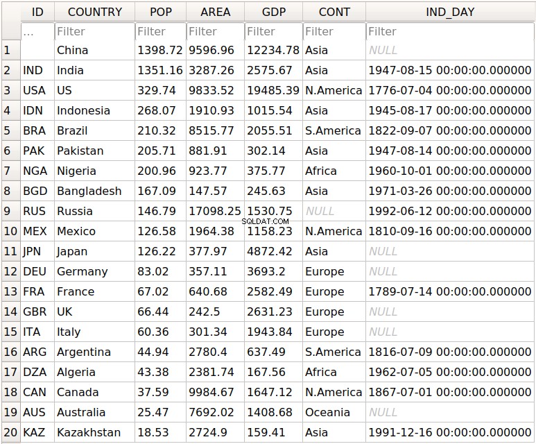
The first column contains the row labels. To omit writing them into the database, pass index=False to .to_sql() . The other columns correspond to the columns of the DataFrame .
There are a few more optional parameters. For example, you can use schema to specify the database schema and dtype to determine the types of the database columns. You can also use if_exists , which says what to do if a database with the same name and path already exists:
if_exists='fail'raises a ValueError and is the default.if_exists='replace'drops the table and inserts new values.if_exists='append'inserts new values into the table.
You can load the data from the database with read_sql() :
>>> df = pd.read_sql('data.db', con=engine, index_col='ID')
>>> df
        COUNTRY      POP      AREA       GDP       CONT    IND_DAY
ID
CHN       China  1398.72   9596.96  12234.78       Asia        NaT
IND       India  1351.16   3287.26   2575.67       Asia 1947-08-15
USA          US   329.74   9833.52  19485.39  N.America 1776-07-04
IDN   Indonesia   268.07   1910.93   1015.54       Asia 1945-08-17
BRA      Brazil   210.32   8515.77   2055.51  S.America 1822-09-07
PAK    Pakistan   205.71    881.91    302.14       Asia 1947-08-14
NGA     Nigeria   200.96    923.77    375.77     Africa 1960-10-01
BGD  Bangladesh   167.09    147.57    245.63       Asia 1971-03-26
RUS      Russia   146.79  17098.25   1530.75       None 1992-06-12
MEX      Mexico   126.58   1964.38   1158.23  N.America 1810-09-16
JPN       Japan   126.22    377.97   4872.42       Asia        NaT
DEU     Germany    83.02    357.11   3693.20     Europe        NaT
FRA      France    67.02    640.68   2582.49     Europe 1789-07-14
GBR          UK    66.44    242.50   2631.23     Europe        NaT
ITA       Italy    60.36    301.34   1943.84     Europe        NaT
ARG   Argentina    44.94   2780.40    637.49  S.America 1816-07-09
DZA     Algeria    43.38   2381.74    167.56     Africa 1962-07-05
CAN      Canada    37.59   9984.67   1647.12  N.America 1867-07-01
AUS   Australia    25.47   7692.02   1408.68    Oceania        NaT
KAZ  Kazakhstan    18.53   2724.90    159.41       Asia 1991-12-16
The parameter index_col specifies the name of the column with the row labels. Note that this inserts an extra row after the header that starts with ID . You can fix this behavior with the following line of code:
>>> df.index.name = None
>>> df
        COUNTRY      POP      AREA       GDP       CONT    IND_DAY
CHN       China  1398.72   9596.96  12234.78       Asia        NaT
IND       India  1351.16   3287.26   2575.67       Asia 1947-08-15
USA          US   329.74   9833.52  19485.39  N.America 1776-07-04
IDN   Indonesia   268.07   1910.93   1015.54       Asia 1945-08-17
BRA      Brazil   210.32   8515.77   2055.51  S.America 1822-09-07
PAK    Pakistan   205.71    881.91    302.14       Asia 1947-08-14
NGA     Nigeria   200.96    923.77    375.77     Africa 1960-10-01
BGD  Bangladesh   167.09    147.57    245.63       Asia 1971-03-26
RUS      Russia   146.79  17098.25   1530.75       None 1992-06-12
MEX      Mexico   126.58   1964.38   1158.23  N.America 1810-09-16
JPN       Japan   126.22    377.97   4872.42       Asia        NaT
DEU     Germany    83.02    357.11   3693.20     Europe        NaT
FRA      France    67.02    640.68   2582.49     Europe 1789-07-14
GBR          UK    66.44    242.50   2631.23     Europe        NaT
ITA       Italy    60.36    301.34   1943.84     Europe        NaT
ARG   Argentina    44.94   2780.40    637.49  S.America 1816-07-09
DZA     Algeria    43.38   2381.74    167.56     Africa 1962-07-05
CAN      Canada    37.59   9984.67   1647.12  N.America 1867-07-01
AUS   Australia    25.47   7692.02   1408.68    Oceania        NaT
KAZ  Kazakhstan    18.53   2724.90    159.41       Asia 1991-12-16
Now you have the same DataFrame object as before.
Note that the continent for Russia is now None instead of nan . If you want to fill the missing values with nan , then you can use .fillna() :
>>> df.fillna(value=float('nan'), inplace=True)
.fillna() replaces all missing values with whatever you pass to value . Here, you passed float('nan') , which says to fill all missing values with nan .
Also note that you didn’t have to pass parse_dates=['IND_DAY'] to read_sql() . That’s because your database was able to detect that the last column contains dates. However, you can pass parse_dates if you’d like. You’ll get the same results.
There are other functions that you can use to read databases, like read_sql_table() and read_sql_query() . Feel free to try them out!
Pickle Files
Pickling is the act of converting Python objects into byte streams. Unpickling is the inverse process. Python pickle files are the binary files that keep the data and hierarchy of Python objects. They usually have the extension .pickle or .pkl .
You can save your DataFrame in a pickle file with .to_pickle() :
>>> dtypes = {'POP': 'float64', 'AREA': 'float64', 'GDP': 'float64',
...           'IND_DAY': 'datetime64'}
>>> df = pd.DataFrame(data=data).T.astype(dtype=dtypes)
>>> df.to_pickle('data.pickle')
Like you did with databases, it can be convenient first to specify the data types. Then, you create a file data.pickle to contain your data. You could also pass an integer value to the optional parameter protocol , which specifies the protocol of the pickler.
You can get the data from a pickle file with read_pickle() :
>>> df = pd.read_pickle('data.pickle')
>>> df
        COUNTRY      POP      AREA       GDP       CONT    IND_DAY
CHN       China  1398.72   9596.96  12234.78       Asia        NaT
IND       India  1351.16   3287.26   2575.67       Asia 1947-08-15
USA          US   329.74   9833.52  19485.39  N.America 1776-07-04
IDN   Indonesia   268.07   1910.93   1015.54       Asia 1945-08-17
BRA      Brazil   210.32   8515.77   2055.51  S.America 1822-09-07
PAK    Pakistan   205.71    881.91    302.14       Asia 1947-08-14
NGA     Nigeria   200.96    923.77    375.77     Africa 1960-10-01
BGD  Bangladesh   167.09    147.57    245.63       Asia 1971-03-26
RUS      Russia   146.79  17098.25   1530.75        NaN 1992-06-12
MEX      Mexico   126.58   1964.38   1158.23  N.America 1810-09-16
JPN       Japan   126.22    377.97   4872.42       Asia        NaT
DEU     Germany    83.02    357.11   3693.20     Europe        NaT
FRA      France    67.02    640.68   2582.49     Europe 1789-07-14
GBR          UK    66.44    242.50   2631.23     Europe        NaT
ITA       Italy    60.36    301.34   1943.84     Europe        NaT
ARG   Argentina    44.94   2780.40    637.49  S.America 1816-07-09
DZA     Algeria    43.38   2381.74    167.56     Africa 1962-07-05
CAN      Canada    37.59   9984.67   1647.12  N.America 1867-07-01
AUS   Australia    25.47   7692.02   1408.68    Oceania        NaT
KAZ  Kazakhstan    18.53   2724.90    159.41       Asia 1991-12-16
read_pickle() returns the DataFrame with the stored data. You can also check the data types:
>>> df.dtypes
COUNTRY            object
POP               float64
AREA              float64
GDP               float64
CONT               object
IND_DAY    datetime64[ns]
dtype: object
These are the same ones that you specified before using .to_pickle() .
As a word of caution, you should always beware of loading pickles from untrusted sources. This can be dangerous! When you unpickle an untrustworthy file, it could execute arbitrary code on your machine, gain remote access to your computer, or otherwise exploit your device in other ways.
Working With Big Data
If your files are too large for saving or processing, then there are several approaches you can take to reduce the required disk space:
- Compress your files
- Choose only the columns you want
- Omit the rows you don’t need
- Force the use of less precise data types
- Split the data into chunks
You’ll take a look at each of these techniques in turn.
Compress and Decompress Files
You can create an archive file like you would a regular one, with the addition of a suffix that corresponds to the desired compression type:
'.gz''.bz2''.zip''.xz'
Pandas can deduce the compression type by itself:
>>>>>> df = pd.DataFrame(data=data).T
>>> df.to_csv('data.csv.zip')
Here, you create a compressed .csv file as an archive. The size of the regular .csv file is 1048 bytes, while the compressed file only has 766 bytes.
You can open this compressed file as usual with the Pandas read_csv() función:
>>> df = pd.read_csv('data.csv.zip', index_col=0,
...                  parse_dates=['IND_DAY'])
>>> df
        COUNTRY      POP      AREA       GDP       CONT    IND_DAY
CHN       China  1398.72   9596.96  12234.78       Asia        NaT
IND       India  1351.16   3287.26   2575.67       Asia 1947-08-15
USA          US   329.74   9833.52  19485.39  N.America 1776-07-04
IDN   Indonesia   268.07   1910.93   1015.54       Asia 1945-08-17
BRA      Brazil   210.32   8515.77   2055.51  S.America 1822-09-07
PAK    Pakistan   205.71    881.91    302.14       Asia 1947-08-14
NGA     Nigeria   200.96    923.77    375.77     Africa 1960-10-01
BGD  Bangladesh   167.09    147.57    245.63       Asia 1971-03-26
RUS      Russia   146.79  17098.25   1530.75        NaN 1992-06-12
MEX      Mexico   126.58   1964.38   1158.23  N.America 1810-09-16
JPN       Japan   126.22    377.97   4872.42       Asia        NaT
DEU     Germany    83.02    357.11   3693.20     Europe        NaT
FRA      France    67.02    640.68   2582.49     Europe 1789-07-14
GBR          UK    66.44    242.50   2631.23     Europe        NaT
ITA       Italy    60.36    301.34   1943.84     Europe        NaT
ARG   Argentina    44.94   2780.40    637.49  S.America 1816-07-09
DZA     Algeria    43.38   2381.74    167.56     Africa 1962-07-05
CAN      Canada    37.59   9984.67   1647.12  N.America 1867-07-01
AUS   Australia    25.47   7692.02   1408.68    Oceania        NaT
KAZ  Kazakhstan    18.53   2724.90    159.41       Asia 1991-12-16
read_csv() decompresses the file before reading it into a DataFrame .
You can specify the type of compression with the optional parameter compression , which can take on any of the following values:
'infer''gzip''bz2''zip''xz'None
The default value compression='infer' indicates that Pandas should deduce the compression type from the file extension.
Here’s how you would compress a pickle file:
>>>>>> df = pd.DataFrame(data=data).T
>>> df.to_pickle('data.pickle.compress', compression='gzip')
You should get the file data.pickle.compress that you can later decompress and read:
>>> df = pd.read_pickle('data.pickle.compress', compression='gzip')
df again corresponds to the DataFrame with the same data as before.
You can give the other compression methods a try, as well. If you’re using pickle files, then keep in mind that the .zip format supports reading only.
Choose Columns
The Pandas read_csv() and read_excel() functions have the optional parameter usecols that you can use to specify the columns you want to load from the file. You can pass the list of column names as the corresponding argument:
>>> df = pd.read_csv('data.csv', usecols=['COUNTRY', 'AREA'])
>>> df
       COUNTRY      AREA
0        China   9596.96
1        India   3287.26
2           US   9833.52
3    Indonesia   1910.93
4       Brazil   8515.77
5     Pakistan    881.91
6      Nigeria    923.77
7   Bangladesh    147.57
8       Russia  17098.25
9       Mexico   1964.38
10       Japan    377.97
11     Germany    357.11
12      France    640.68
13          UK    242.50
14       Italy    301.34
15   Argentina   2780.40
16     Algeria   2381.74
17      Canada   9984.67
18   Australia   7692.02
19  Kazakhstan   2724.90
Now you have a DataFrame that contains less data than before. Here, there are only the names of the countries and their areas.
Instead of the column names, you can also pass their indices:
>>>>>> df = pd.read_csv('data.csv',index_col=0, usecols=[0, 1, 3])
>>> df
COUNTRY AREA
CHN China 9596.96
IND India 3287.26
USA US 9833.52
IDN Indonesia 1910.93
BRA Brazil 8515.77
PAK Pakistan 881.91
NGA Nigeria 923.77
BGD Bangladesh 147.57
RUS Russia 17098.25
MEX Mexico 1964.38
JPN Japan 377.97
DEU Germany 357.11
FRA France 640.68
GBR UK 242.50
ITA Italy 301.34
ARG Argentina 2780.40
DZA Algeria 2381.74
CAN Canada 9984.67
AUS Australia 7692.02
KAZ Kazakhstan 2724.90
Expand the code block below to compare these results with the file 'data.csv' :
,COUNTRY,POP,AREA,GDP,CONT,IND_DAY
CHN,China,1398.72,9596.96,12234.78,Asia,
IND,India,1351.16,3287.26,2575.67,Asia,1947-08-15
USA,US,329.74,9833.52,19485.39,N.America,1776-07-04
IDN,Indonesia,268.07,1910.93,1015.54,Asia,1945-08-17
BRA,Brazil,210.32,8515.77,2055.51,S.America,1822-09-07
PAK,Pakistan,205.71,881.91,302.14,Asia,1947-08-14
NGA,Nigeria,200.96,923.77,375.77,Africa,1960-10-01
BGD,Bangladesh,167.09,147.57,245.63,Asia,1971-03-26
RUS,Russia,146.79,17098.25,1530.75,,1992-06-12
MEX,Mexico,126.58,1964.38,1158.23,N.America,1810-09-16
JPN,Japan,126.22,377.97,4872.42,Asia,
DEU,Germany,83.02,357.11,3693.2,Europe,
FRA,France,67.02,640.68,2582.49,Europe,1789-07-14
GBR,UK,66.44,242.5,2631.23,Europe,
ITA,Italy,60.36,301.34,1943.84,Europe,
ARG,Argentina,44.94,2780.4,637.49,S.America,1816-07-09
DZA,Algeria,43.38,2381.74,167.56,Africa,1962-07-05
CAN,Canada,37.59,9984.67,1647.12,N.America,1867-07-01
AUS,Australia,25.47,7692.02,1408.68,Oceania,
KAZ,Kazakhstan,18.53,2724.9,159.41,Asia,1991-12-16
You can see the following columns:
- The column at index
0contains the row labels. - The column at index
1contains the country names. - The column at index
3contains the areas.
Simlarly, read_sql() has the optional parameter columns that takes a list of column names to read:
>>> df = pd.read_sql('data.db', con=engine, index_col='ID',
...                  columns=['COUNTRY', 'AREA'])
>>> df.index.name = None
>>> df
        COUNTRY      AREA
CHN       China   9596.96
IND       India   3287.26
USA          US   9833.52
IDN   Indonesia   1910.93
BRA      Brazil   8515.77
PAK    Pakistan    881.91
NGA     Nigeria    923.77
BGD  Bangladesh    147.57
RUS      Russia  17098.25
MEX      Mexico   1964.38
JPN       Japan    377.97
DEU     Germany    357.11
FRA      France    640.68
GBR          UK    242.50
ITA       Italy    301.34
ARG   Argentina   2780.40
DZA     Algeria   2381.74
CAN      Canada   9984.67
AUS   Australia   7692.02
KAZ  Kazakhstan   2724.90
Again, the DataFrame only contains the columns with the names of the countries and areas. If columns is None or omitted, then all of the columns will be read, as you saw before. The default behavior is columns=None .
Omit Rows
When you test an algorithm for data processing or machine learning, you often don’t need the entire dataset. It’s convenient to load only a subset of the data to speed up the process. The Pandas read_csv() and read_excel() functions have some optional parameters that allow you to select which rows you want to load:
skiprows: either the number of rows to skip at the beginning of the file if it’s an integer, or the zero-based indices of the rows to skip if it’s a list-like objectskipfooter: the number of rows to skip at the end of the filenrows: the number of rows to read
Here’s how you would skip rows with odd zero-based indices, keeping the even ones:
>>>>>> df = pd.read_csv('data.csv', index_col=0, skiprows=range(1, 20, 2))
>>> df
COUNTRY POP AREA GDP CONT IND_DAY
IND India 1351.16 3287.26 2575.67 Asia 1947-08-15
IDN Indonesia 268.07 1910.93 1015.54 Asia 1945-08-17
PAK Pakistan 205.71 881.91 302.14 Asia 1947-08-14
BGD Bangladesh 167.09 147.57 245.63 Asia 1971-03-26
MEX Mexico 126.58 1964.38 1158.23 N.America 1810-09-16
DEU Germany 83.02 357.11 3693.20 Europe NaN
GBR UK 66.44 242.50 2631.23 Europe NaN
ARG Argentina 44.94 2780.40 637.49 S.America 1816-07-09
CAN Canada 37.59 9984.67 1647.12 N.America 1867-07-01
KAZ Kazakhstan 18.53 2724.90 159.41 Asia 1991-12-16
In this example, skiprows is range(1, 20, 2) and corresponds to the values 1 , 3 , …, 19 . The instances of the Python built-in class range behave like sequences. The first row of the file data.csv is the header row. It has the index 0 , so Pandas loads it in. The second row with index 1 corresponds to the label CHN , and Pandas skips it. The third row with the index 2 and label IND is loaded, and so on.
If you want to choose rows randomly, then skiprows can be a list or NumPy array with pseudo-random numbers, obtained either with pure Python or with NumPy.
Force Less Precise Data Types
If you’re okay with less precise data types, then you can potentially save a significant amount of memory! First, get the data types with .dtypes de nuevo:
>>> df = pd.read_csv('data.csv', index_col=0, parse_dates=['IND_DAY'])
>>> df.dtypes
COUNTRY            object
POP               float64
AREA              float64
GDP               float64
CONT               object
IND_DAY    datetime64[ns]
dtype: object
The columns with the floating-point numbers are 64-bit floats. Each number of this type float64 consumes 64 bits or 8 bytes. Each column has 20 numbers and requires 160 bytes. You can verify this with .memory_usage() :
>>> df.memory_usage()
Index      160
COUNTRY    160
POP        160
AREA       160
GDP        160
CONT       160
IND_DAY    160
dtype: int64
.memory_usage() returns an instance of Series with the memory usage of each column in bytes. You can conveniently combine it with .loc[] and .sum() to get the memory for a group of columns:
>>> df.loc[:, ['POP', 'AREA', 'GDP']].memory_usage(index=False).sum()
480
This example shows how you can combine the numeric columns 'POP' , 'AREA' , and 'GDP' to get their total memory requirement. The argument index=False excludes data for row labels from the resulting Series objeto. For these three columns, you’ll need 480 bytes.
You can also extract the data values in the form of a NumPy array with .to_numpy() or .values . Then, use the .nbytes attribute to get the total bytes consumed by the items of the array:
>>> df.loc[:, ['POP', 'AREA', 'GDP']].to_numpy().nbytes
480
The result is the same 480 bytes. So, how do you save memory?
In this case, you can specify that your numeric columns 'POP' , 'AREA' , and 'GDP' should have the type float32 . Use the optional parameter dtype to do this:
>>> dtypes = {'POP': 'float32', 'AREA': 'float32', 'GDP': 'float32'}
>>> df = pd.read_csv('data.csv', index_col=0, dtype=dtypes,
...                  parse_dates=['IND_DAY'])
The dictionary dtypes specifies the desired data types for each column. It’s passed to the Pandas read_csv() function as the argument that corresponds to the parameter dtype .
Now you can verify that each numeric column needs 80 bytes, or 4 bytes per item:
>>>>>> df.dtypes
COUNTRY object
POP float32
AREA float32
GDP float32
CONT object
IND_DAY datetime64[ns]
dtype: object
>>> df.memory_usage()
Index 160
COUNTRY 160
POP 80
AREA 80
GDP 80
CONT 160
IND_DAY 160
dtype: int64
>>> df.loc[:, ['POP', 'AREA', 'GDP']].memory_usage(index=False).sum()
240
>>> df.loc[:, ['POP', 'AREA', 'GDP']].to_numpy().nbytes
240
Each value is a floating-point number of 32 bits or 4 bytes. The three numeric columns contain 20 items each. In total, you’ll need 240 bytes of memory when you work with the type float32 . This is half the size of the 480 bytes you’d need to work with float64 .
In addition to saving memory, you can significantly reduce the time required to process data by using float32 instead of float64 in some cases.
Use Chunks to Iterate Through Files
Another way to deal with very large datasets is to split the data into smaller chunks and process one chunk at a time. If you use read_csv() , read_json() or read_sql() , then you can specify the optional parameter chunksize :
>>> data_chunk = pd.read_csv('data.csv', index_col=0, chunksize=8)
>>> type(data_chunk)
<class 'pandas.io.parsers.TextFileReader'>
>>> hasattr(data_chunk, '__iter__')
True
>>> hasattr(data_chunk, '__next__')
True
chunksize defaults to None and can take on an integer value that indicates the number of items in a single chunk. When chunksize is an integer, read_csv() returns an iterable that you can use in a for loop to get and process only a fragment of the dataset in each iteration:
>>> for df_chunk in pd.read_csv('data.csv', index_col=0, chunksize=8):
...     print(df_chunk, end='\n\n')
...     print('memory:', df_chunk.memory_usage().sum(), 'bytes',
...           end='\n\n\n')
...
        COUNTRY      POP     AREA       GDP       CONT     IND_DAY
CHN       China  1398.72  9596.96  12234.78       Asia         NaN
IND       India  1351.16  3287.26   2575.67       Asia  1947-08-15
USA          US   329.74  9833.52  19485.39  N.America  1776-07-04
IDN   Indonesia   268.07  1910.93   1015.54       Asia  1945-08-17
BRA      Brazil   210.32  8515.77   2055.51  S.America  1822-09-07
PAK    Pakistan   205.71   881.91    302.14       Asia  1947-08-14
NGA     Nigeria   200.96   923.77    375.77     Africa  1960-10-01
BGD  Bangladesh   167.09   147.57    245.63       Asia  1971-03-26

memory: 448 bytes


       COUNTRY     POP      AREA      GDP       CONT     IND_DAY
RUS     Russia  146.79  17098.25  1530.75        NaN  1992-06-12
MEX     Mexico  126.58   1964.38  1158.23  N.America  1810-09-16
JPN      Japan  126.22    377.97  4872.42       Asia         NaN
DEU    Germany   83.02    357.11  3693.20     Europe         NaN
FRA     France   67.02    640.68  2582.49     Europe  1789-07-14
GBR         UK   66.44    242.50  2631.23     Europe         NaN
ITA      Italy   60.36    301.34  1943.84     Europe         NaN
ARG  Argentina   44.94   2780.40   637.49  S.America  1816-07-09

memory: 448 bytes


        COUNTRY    POP     AREA      GDP       CONT     IND_DAY
DZA     Algeria  43.38  2381.74   167.56     Africa  1962-07-05
CAN      Canada  37.59  9984.67  1647.12  N.America  1867-07-01
AUS   Australia  25.47  7692.02  1408.68    Oceania         NaN
KAZ  Kazakhstan  18.53  2724.90   159.41       Asia  1991-12-16

memory: 224 bytes
In this example, the chunksize is 8 . The first iteration of the for loop returns a DataFrame with the first eight rows of the dataset only. The second iteration returns another DataFrame with the next eight rows. The third and last iteration returns the remaining four rows.
iterator=True to force the Pandas read_csv() function to return an iterator object instead of a DataFrame objeto.
In each iteration, you get and process the DataFrame with the number of rows equal to chunksize . It’s possible to have fewer rows than the value of chunksize in the last iteration. You can use this functionality to control the amount of memory required to process data and keep that amount reasonably small.
Conclusión
You now know how to save the data and labels from Pandas DataFrame objects to different kinds of files. You also know how to load your data from files and create DataFrame objects.
You’ve used the Pandas read_csv() and .to_csv() methods to read and write CSV files. You also used similar methods to read and write Excel, JSON, HTML, SQL, and pickle files. These functions are very convenient and widely used. They allow you to save or load your data in a single function or method call.
You’ve also learned how to save time, memory, and disk space when working with large data files:
- Compress or decompress files
- Choose the rows and columns you want to load
- Use less precise data types
- Split data into chunks and process them one by one
You’ve mastered a significant step in the machine learning and data science process! If you have any questions or comments, then please put them in the comments section below.